R3-[Q-Shape] - Research: Qualitative Spatial Reasoning
Complexity of constraint-based reasoning algorithms for ternary calculi
Qualitative knowledge about relative distance and orientation can be expressed in form of ternary point relations. Results by Scivos and Nebel showed that Freksa's Double Cross calculus is ![]() -hard [SN01].
-hard [SN01].
The calculus we will use for our investigations, the Ternary Point Configuration Calculus (TPCC) [MNF03], is derived from the Double Cross calculus [Fre92] and is developed under the premises being suitable for robot navigation human machine interaction.
We investigate the question whether ternary point configuration calculi are useful for polynomial but incomplete reasoning. Therefore we investigate properties and complexity issues of several algorithms calculating fix points within TPCC constraint systems.
A prerequisite to using the standard constraint algorithms, especially the Ladkin and Reinefeld's algorithm [LR92] extended for ternary relations [IC00], is to express the calculi in terms of relation algebras in the sense of Tarski [LM94]. But since the TPCC-Calculus is not closed under the transformations and under the composition we can not use this scheme.
However, simple path-based inferences can be performed using the following scheme. The two last relations of a path are composed. Then the reference system is incrementally moved towards the beginning of the path in form of a backward chaining. For an example see the Aibo-Example page. Here we will look at four different algorithms calculating a fix point for a given constraint system with ternary relations with more general methods. The result is some sort of hyper-arc-consistency.
In the following, we denote the set of objects involved with O and we define a triple of objects x,y,z ∈ O as <x,y,z>. In the following we may refer to a triple as well as node or point configuration. We name the set of all possible valid triples ![]() with n objects given. Thus the number of valid nodes is
with n objects given. Thus the number of valid nodes is 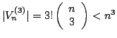 . For each triple we have a number of
 ![]() possible relations, what is the number of base relations of the TPCC calculus. The constraints for a single configuration are summarized in
possible relations, what is the number of base relations of the TPCC calculus. The constraints for a single configuration are summarized in ![]() and the union of all constraints over all nodes is named C. The rules given by the TPCC for transformation are refered as
and the union of all constraints over all nodes is named C. The rules given by the TPCC for transformation are refered as ![]() and for composition as
and for composition as ![]() .
.
Algorithm 1 is a naive implementation like the one proposed by Montanari [Mon74], Algorithm 2 is similar to the first one, but with recursive precalculations of depth two on all initially given constraints. Method 3 shows an extended version following Mackworth [Mac77], listing all changes in a queue, and Algorithm 4 is a method propagating all effects of the initially given constraints and the emerging changes recursively.
Algorithm 1 – Naive fix point calculation
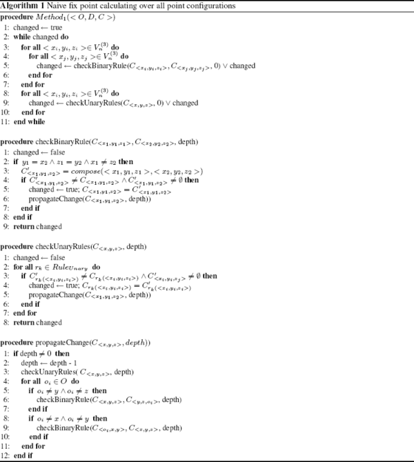
The naive implementation (Alg. 1) checks all combinations of triples whether they have a composition and calculating the emerging changes on the dependant relations. This loop is iterated until a fix point is reached. With the approximation of ![]() we have
we have ![]() for the inner loop, with c denoting the costs for calculating the composition of two configurations. With
for the inner loop, with c denoting the costs for calculating the composition of two configurations. With ![]() follows
follows ![]() . Following [Mon74] the outer loop is executed maximal linear in the number of nodes times the maximum domain size. This results in
. Following [Mon74] the outer loop is executed maximal linear in the number of nodes times the maximum domain size. This results in![]() . Thus an overall complexity of
. Thus an overall complexity of ![]() follows.
follows.
Algorithm 2 – Recursive Propagation with bounded depth
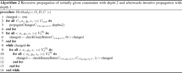
In the case of Algorithm 2 the recursive propagation of all initially given constraints with depth two takes ![]() . The loop for propagating the changes with depth one is executed n³a times in the worst case. The propagation itself takes
. The loop for propagating the changes with depth one is executed n³a times in the worst case. The propagation itself takes ![]() . This results in a worst case complexity of
. This results in a worst case complexity of ![]() . This is worse than Algorithm 1, but in the average the loop is called only a few times (≤n), which leads to
. This is worse than Algorithm 1, but in the average the loop is called only a few times (≤n), which leads to ![]() .
.
Algorithm 3 – AC-3/PC-2 like algorithm
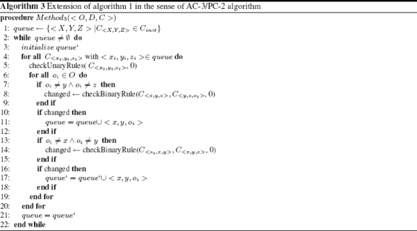
Algorithm 3 is modified in the sense of Mackworth listing all changes occurring within a loop and revising only these in the next loop. A first investigation resulted in a complexity of ![]() [DM04]. Having a closer look at subprogram checkUnaryRules revealed a lower complexity of
[DM04]. Having a closer look at subprogram checkUnaryRules revealed a lower complexity of ![]() [MR05]. The subprogram returns TRUE, if by using the transformation tables, a constraint is replaced by a stricter one.. Analogically, the subprogram checkBinaryRules returns TRUE, if by using the composition table a constraint is replaced by a stricter constraint. The variable changed is true if and only if for one node at least one base relation has been excluded. If this happens, the queue' has been extended by a new element. For that reason, we have in the worst case no more than
[MR05]. The subprogram returns TRUE, if by using the transformation tables, a constraint is replaced by a stricter one.. Analogically, the subprogram checkBinaryRules returns TRUE, if by using the composition table a constraint is replaced by a stricter constraint. The variable changed is true if and only if for one node at least one base relation has been excluded. If this happens, the queue' has been extended by a new element. For that reason, we have in the worst case no more than ![]() nodes in the queue (for each
nodes in the queue (for each ![]() with
with ![]() ). In the iteration of the loop each element leads to n calls of checkBinaryRules. Therefore the complexity of this algorithm is
). In the iteration of the loop each element leads to n calls of checkBinaryRules. Therefore the complexity of this algorithm is ![]() .
.
Algorithm 4 – Recursive propagation
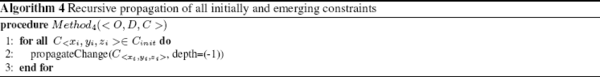
The recursive algorithm (Alg. 4) propagates all changes originating in the initially given constraints (≤k∗n with a constant k). The maximum depth is bounded in the number of nodes ![]() . Executing the function propagateChange(.) with depth one takes
. Executing the function propagateChange(.) with depth one takes ![]() . The recursive call with depth >1 leads to 2nc calls of propagateChange(.) plus an additional overhead of
. The recursive call with depth >1 leads to 2nc calls of propagateChange(.) plus an additional overhead of ![]() . This can be summarized with
. This can be summarized with ![]() resulting in a term exponential in the maximum number of nodes, what is
resulting in a term exponential in the maximum number of nodes, what is ![]() .
.
Bibliography
[DM04]: F. Dylla and R. Moratz. Emprical complexity issues of practical qualitative spatial reasoning about relative position. Workshop on Spatial and Temporal Reasoning, ECAI 2004, 2004.
[Fre92]: C. Freksa. Using Orientation Information for Qualitative Spatial Reasoning. In A. U. Frank, I. Campari, and U. Formentini, editors, Theories and Methods of Spatial-Temporal Reasoning in Geographic Space, pages 162-178. Springer, Berlin, 1992.
[IC00]: A. Isli and A. Cohn. Qualitative spatial reasoning: A new approach to cyclic ordering of 2d orientation. Artificial Intelligence, 122:137-187, 2000.
[LM94]: P Ladkin and R Maddux. On binary constraint problems. Journal of the Association for Computing Machinery, 41(3):435-469, 1994.
[LR92]: P Ladkin and A Reinefeld. Effective solution of qualitative constraint problems. Artificial Intelligence, 57:105-124, 1992.
[Mac77] A K Mackworth. Consistency in networks of relations. Artificial Intelligence, 8:99-118, 1977.
[MNF03]: R. Moratz, B. Nebel, and C. Freksa. Qualitative spatial reasoning about relative position: The tradeoff between strong formal properties and successful reasoning about route graphs. In C. Freksa, W. Brauer, C. Habel, and K.F. Wender, editors, Lecture Notes in Artificial Intelligence 2685: Spatial Cognition III, pages 385-400. Springer Verlag, Berlin/Heidelberg, 2003.
[MR05]: R. Moratz, and M. Ragni. Qualitative spatial reasoning about relative point positions. (submitted), 2005.
[Mon74]: U. Montanari. Networks of constraints: Fundamental properties and applications to picture processing. Information Sciences, 7:95-132, 1974.
[SN01]: A. Scivos and B. Nebel. Double-crossing: Decidability and computational complexity of a qualitative calculus for navigation. In COSIT 2001, Berlin, 2001. Springer.